
Kepler.gl is a powerful open source geospatial analysis tool for large-scale data sets.
Playback
Follow these steps to create a playback video of an event:
Add a filter based on a time-related field, like timestamp. For GeoJson, property field should contain a timestamp entry.
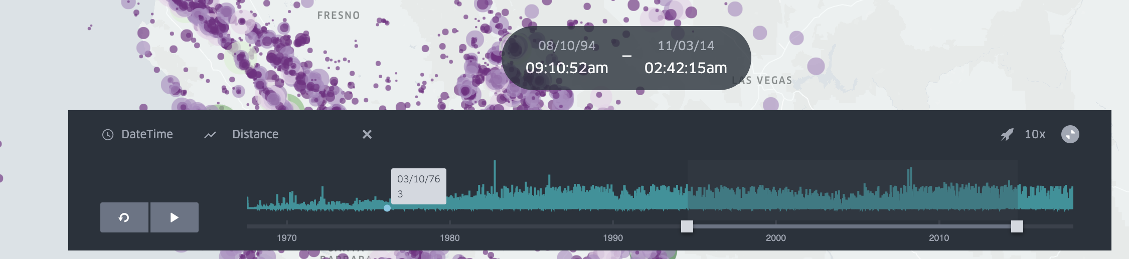
The playback window will appear on the bottom of the map. The bars are distribution graphs of all data points by time. Select the desired rolling time window:

- Press play to start the video. Click on the speed value and select/input your desired value 1x, 2x, 4x on the top right to change the playback speed.

- Choose custom y axis. You can click Select Y Axis to change the default distribution graph to a timeseries of the selected column. An example use of this function is to show a distance vs. time graph of a given trip.
Animation window modes
Use the animation window control on the playback bar to choose how the time range moves during playback:
- Moving Time Window (default): a fixed-length window slides forward. Features appear while their time falls inside the window, then disappear when the window moves past them.
- Incremental Time Window: the window start stays fixed and only the end advances. Features accumulate once their timestamp is reached and stay visible until the animation loops or resets (then the window shrinks again and accumulation starts over). Use this when you have a single timestamp field and want cumulative playback (similar to “accumulate” in other GIS tools).
- Step by Interval: the window is one histogram bin wide and jumps to the next bin on each frame. Dragging the histogram selects a single bin; the brush stays locked to that bin while this mode is on. Wheel-resizing the time window is turned off so the selection cannot stretch across bins.
Start and end time (duration)
By default, playback uses a single timestamp field: a feature is visible only while that instant falls inside the current time window (see Animation window modes above).
To keep features visible for a whole time span (service coverage, deployments, availability windows), add a time filter on the start timestamp, then optionally choose an End time field in the filter panel. A feature stays on the map while the playback window overlaps [start, end]. Rows with a missing end time are treated as still active. The timeline histogram counts a feature in every bin that overlaps its start–end range.
End time is available only on a time filter that is not synced across datasets. If you use Time Filter Sync, clear the extra datasets first, then set End time.
Incremental Time Window and End time solve different problems: use Incremental when each feature is a single instant and you want them to accumulate; use End time when each feature has its own start–end duration.
Zoom & precision controls
The enlarged timeline now lets you stay focused on the portion that matters:
- Use the mouse wheel to resize the window under the cursor, and pinch (or hold Ctrl on Windows/Linux or ⌘ on macOS while scrolling) to zoom the full timeline.
- A lightweight "Showing" bar appears whenever the full range is narrowed—click Reset to return to the original domain.
- Hold Ctrl (Windows/Linux) or ⌘ (macOS) and press the arrow keys to pan left/right, with Shift for bigger steps.